Protests by British university economic students, whose demonstrations have been backed by prominent academics, highlight the notion that economic education is dominated by theories that defy practical applications and applications that can not predict, prevent or ameliorate periodic crises. Students learn economics from unverified theories, many contradicting each other, which leads to a confused understanding of the discipline and complicated approaches to resolve problems. Adding to the dilemma is that textbooks in Middle Schools, High Schools and universities lack updates with recent knowledge and contain dubious propositions. It is time to examine several propositions that are prominent but seem dubious. This examination is not absolute, is intended to arouse discussion, and, hopefully, serve to gauge if they should be restated or expunged from current academic learning, textbooks, and public discourse.
(1) Keynes Multiplier
(2) Laffer curve
(3) Philips Curve
(4) Disposable income
(5) Okuns Law
Keynes GDP Multiplier
One explanation of the Keynesian "multiplier" is from https://wiki.ubc.ca/Keynesian_Multiplier :
The Keynesian multiplier works as follows. Marginal propensity to consume (MPC) = 0.8, when people get an extra dollar of income, and spend 80 cents of it. If the government increases expenditure by 1 dollar on a good produced by agent A, this dollar becomes A's income. As MPC = 0.8, A will spend 80 cents of this extra income on something it wants to consume. Suppose A spends the 80 cents on a good produced by B, then B would have an extra income of 80 cents. B would then spend 0.8 of this 80 cents, ie, 64 cents, on something else. This 64 cents becomes someone else's income, and this someone will spend 0.8 of it. The process repeats itself. The GDP added to the economy is the sum of all the spending, 1 + 0.8 + 0.64 + 0.512 + ... which has a larger effect than the 1 dollar that the government originally spent. In other words, the government spending is "multiplied". Mathematically, the sum 1 + 0.8 + 0.64 + ... is a geometric series. When you sum them up, it takes the form 1/1-MPC. For MPC = 0.8, the effect of the government spending is multiplied 5 times.
Can a fiscal multiplier of >1 exist? Has Keynes been misinterpreted?
Many economists have highlighted the ambiguities in the Keynes multiplier, but it remains accepted by a large segment of the economic community. A simple observation demonstrates its failure - the assertion that, if the velocity of money is unity, one dollar can produce more than one dollar of goods in one production cycle, defies basic logic.
When the government uses deficit spending to buy goods that are produced by A, then A has funds for replenishing the inventory. If A spends on goods from B and does not use the funds to repeat production, then production for A’s inventory ceases (future GDP drops) and A’s spending initiates an equivalent production by producer B (future GDP increases). At no time does added production exceed the original spending.
Imagine a hypothetical system where the cost of goods produced (N) is in balance with the price of goods sold (P), and the money (M) available to purchase the goods. The purchases of all goods continually generate new cycles of production of the same amount of goods. Add the new dollars (d) to the economic system. If all goods available remain at N, then absorbing the added spending dictates an increase in prices. If entrepreneurs use the added dollars to produce additional dollars of goods, the economy is in balance again - (N+d) cost of goods is in balance with (P+d) price of goods and the available money (M+d) to purchase the goods. After (N+d) goods are sold in one round of spending, a new production cycle of (N+d) goods starts. Until more money enters the money supply, each production cycle cannot produce more than (N+d) goods.
The concept that A buys goods from B, which allows B to buy goods from C, and so forth, and that this increases GDP by more than the initial investment is implausible. Each is buying already produced goods with sufficient funds to purchase all the goods from the present production cycle. After all the goods have been purchased, others will be left with funds that are equal to the original expenditure. The GDP will only increase if these funds are invested in new production and that increase will, at maximum, be equal to the original expenditure,
Taken at face value, the Keynesian Multiplier hits a theoretical inconsistency; when MPC = 1, the multiplication becomes infinite, and the era of abundance has been reached. Actually a MPC = 1 signifies that, if the total of the original investment is spent, reinvested, and continues to be totally spent and reinvested, then, after an infinite number of rounds of spending, the total contribution to GDP of this investment (not the value of GDP) during the infinite period will reach infinity -- not surprising.
Rather than being a "multiplier," the formula is actually a "divider." Keynes’ formula states that, if not all available spending is used to purchase goods in a production cycle, less goods will be manufactured in succeeding cycles. Eventually, the public will no longer need these specific goods, and manufacturing of those goods will cease. Let MPC=0.8 in the investment series described above, and, with each investment cycle, the investment is reduced by 20% until it becomes nil and the company stops producing from the original investment. Instead of investment being multiplied by 0.8, investment is reduced by 0.2. If MPC =1, then investment is entirely repeated in each investment cycle and after an infinite number of cycles, total investment reaches infinity. The formula becomes logical and has no indeterminate value.
Keynes' "investment multiplier" only describes the way the system works - sell the goods in one investment cycle, and, if there are additions to demand from additions to the money supply, start a new investment cycle that is greater than the previous cycle by the added demand and increased money supply. The renowned economist iterated in mathematical terms what all adequate company managers know - if you turn over inventory quickly and replace it with new inventory, the enterprise can earn a lot of bucks.
Laffer Curve
The Laffer Curve graphs a hypothetical relationship between tax rates and tax revenue collected by a government. Arthur Laffer, one of President Reagan's Economic Policy advisors, credits Ibn Khaldun, a 14th century philosopher, as being the originator of the curve. The Arab philosopher wrote: "It should be known that at the beginning of the dynasty, taxation yields large revenue from small assessments. At the end of the dynasty, taxation yields small revenue from large assessments."
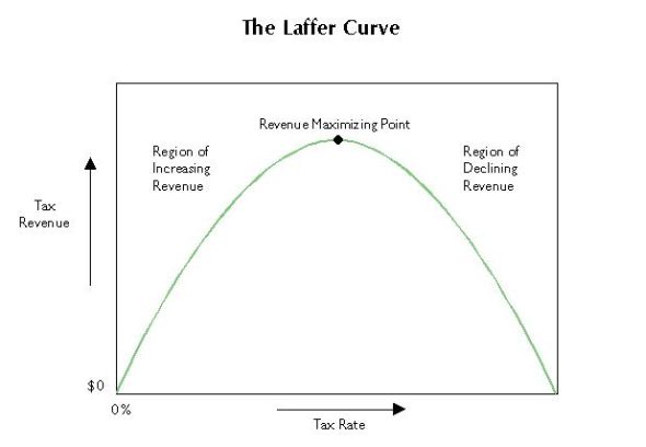
The Laffer curve does not specify a desired tax rate; it simply states that tax revenues increase as the tax rate increases until the tax rate reaches a level where the tax revenue will decrease. Is this a correct curve, and is it relevant?
Is the Laffer curve correct?
Consider the number of different types of taxes, the number of different tax schedules, the number of combinations that combine private spending and government spending into total spending, and the different types of government spending, and a representative curve of government income as a function of tax rate becomes impossible to conceive.
Take an extreme hypothetical case, where the government taxes close to 100 percent, yes 100 percent. There is a caveat - the standard deduction is a percentage of gross income, which allows each earner to have sufficient income for basic and other needs. Government spending of the tax revenue is calculated to increase employment and clear the shelves of all manufactured goods. Corporate income, consumer spending, and GDP remain the same regardless of the tax rate. However, government income increases as the tax rate increases, redistribution of income increases, and unemployment is designed to be minimized.
Is the Laffer curve relevant?
Ibn Khaldun wrote his treatise for a 14th century despot, who wanted to maximize his revenue at the expense of his subjects. The federal government is not a unique person; it is a public institution that has neither need nor want to maximize revenue. It is impossible to ascertain the tax rate that maximizes revenue and there is no benefit to learn that hallowed number.
Conclusion: The Laffer Curve has no theoretical support and is no guide for tax policy. The optimum tax depends upon the particular economic moment and needs for government spending.
Philips Curve
The Philips curve has had several transitions from its original concept. Its inception started from a paper in 1958 titled The Relation between Unemployment and the Rate of Change of Money Wage Rates in the United Kingdom, 1861-1957, which William Phillips, a New Zealand born economist, published in the quarterly journal Economica. Phillips described an apparent inverse relationship between wage changes and unemployment in the British economy during a one hundred year period. Because wage and price inflation seemed to move together, economists determined there must be a link between inflation and unemployment; when inflation was high, unemployment was low, and vice-versa. Historical data during the 1960s appeared to support the theory.
Ref: https://www.frbsf.org/education/publications/doctor-econ/2008/march/phillips-curve-inflation/
Support, but not prove. Statistical coincidence is not proof.
Another statistical match.
Plot defense spending during the same years and a similar curve emerges, where inflation is related to increased defense spending.
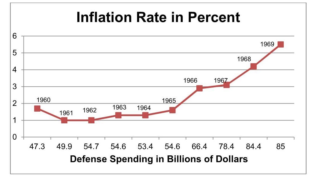
Data from: https://www.macrotrends.net/countries/USA/united-states/militaryspending-defense-budget
During the 60s, the United States had increased defense spending, which increased employment without increaseing consumer goods production. Add the 1964 tax cut to the increases in defense spending and we have increased demand without increased supply. Could this have caused the inflation?
Historical data during the period from 1990-1999, which shows inflation and the unemployment rate decreasing together, refutes the Philips curve.
Ref: Federal Reserve Bank of San Francisco
http://www.frbsf.org/education/publications/doctor-econ/2008/march/phillips-curve-inflation
The record low unemployment and simultaneous low inflation rates during the late Obama and early Trump administrations also demonstrate the error of the Philips curve.
An explanation for why inflation sometimes occurs when unemployment decreases may be more due to the euphoria in an expanding economy. As the economy looks bright, the bright start to borrow, which raises asset values and consumer demand. If the money supply creates demand that swells beyond production capacity, then prices are sure to rise. In addition, if the government continues to run deficits, which usually transfers savings to demand, the pressure on prices increases. During the Clinton administration, the government ran surpluses, which lowered demand and maintained prices.
Thus, it is incorrect to attribute decreasing unemployment to increasing inflation and vice-versa; it is the optimistic market and uncontrolled money supply expansion that causes the inflation. Actually, as the industrial base and employment expand, costs should decrease — economies of scale grow and fixed costs become a lesser cost of each production item, at least until the marginal revenue for each new worker starts to decrease.
Philips has thrown a curveball.
Disposable income
Disposable income is defined in textbooks as total personal income minus total personal taxes.
This may be true, but analysis shows it is meaningless. The definition makes it appear that taxation lessens disposable income, and taxes remove spending from the economy.
Government spending transfers taxes back to the economy and provides income to workers. Other than profits made by corporations from government spending, interest payments (which may become another person’s income), foreign assistance that does not require payback or purchase of U.S. goods, and maintaining U.S. facilities in foreign countries, government spending from taxation winds up in the pockets of others as income. Individuals may have their disposable income reduced by taxes, and disposable income at one moment may be “income minus taxes,” but the disposable income of the entire population, in the long run, eventually remains almost the same as the original total personal income.
As a simple example, let us have the tax revenue used to support the income of government workers. In effect, disposable income has been entirely transferred from the private sector to the public sector, but remains the same. The civil service workers also pay taxes and their taxes may support wages in a defense industry. Continue through continuous quick cycles of pay-as-you-go-taxation and government spending and we find that disposable income (DI) for the entire population is almost always equal to original income. The regeneration of taxes and income follows the geometric series shown below, where t, a number <1, is the tax rate.
DI = (1-t) + (t- t2) + (t2-t3) + … (tn-1-tn) = (1-t) (1 + t + t2 + t3 +…tn)
If n goes to infinity, the equation becomes (1-t) / (1-t) = 1.
During a fiscal year, the government cannot, ad infinitum, invest all tax revenue, but can make, say, two turnovers of tax revenue to spending. DI then equals (1-t) + (t-t2) + (t2-t3), which becomes DI= 1-t3.
If t=0.2, then DI = .992, and almost all the original personal income is available as disposable income.
It is true that disposable income (DI) is personal income (PI) less taxes, but part of the personal income is derived from spent taxes.
Using real numbers, for the year 2018, a rough analysis shows that Disposable Income does not equal total personal income minus total personal taxes.
With figures in billions of dollar, the Bureau of Economic analysis (BEA) has
Personal Income: 18,760
Personal consumption expenditures: 14,759
Statista at https://www.statista.com/statistics/710209/us-disposable-income/ has
Disposable income: 14,556, almost equal to personal consumption expenditures.
The Tax Policy Center at https://www.taxpolicycenter.org/briefing-book/what-are-sources-revenue-federal-government shows
Federal revenue: 3,115 from personal, FICA, and excise taxes
The Tax Administration at https://www.taxadmin.org/2019-state-tax-revenue shows
Total revenue from all state taxes: 1,090
Subtracting all taxes (4,205) from Personal Income (18,760) gives
Disposable income at 14,555, the same as Statista’s value and close to personal consumption expenditures of 14,759.
Wait, this is not the total story. Personal expenditures are not entirely personal consumption; other expenditures absorb income. From St. Louis Fed, these are:
Personal saving: 1,205
Personal Consumption of fixed capital: 609
Financial obligations — rent, auto leases, homeowners' insurance, and property taxes — 2,183
Household Debt Service Payments: 1,456
These expenditures add to $5.453 trillion, some of which leads to income for others. The exact amount that creates income is not easily calculated.
Total expenditures (Disposable Income) are the latter expenditures plus consumer spending, which totals $20,212 trillion. Where does the income for these surplus expenditures arise; they are partially recirculated income, but mainly come from government spending of taxes, which includes income, FICA, excise, corporate and other miscellaneous taxes, some government income from federal businesses, and deficit spending.
In 2018 and 2019 fiscal years, the government averaged $4.35 trillion in spending, much of which served as Disposable Income.
Disposable income, as defined in textbooks as total personal income minus total personal taxes may be true, but analysis shows it is meaningless.
Okun’s Law
Former Federal Reserve Chairman, Ben Bernanke summarized Okun's Law:
Okun noted that, because of ongoing increases in the size of the labor force and in the level of productivity, real GDP growth close to the rate of growth of its potential is normally required, just to hold the unemployment rate steady. To reduce the unemployment rate, therefore, the economy must grow at a pace above its potential.
More specifically, according to [the] currently accepted versions of Okun's law, to achieve a 1 percentage point decline in the unemployment rate in the course of a year, real GDP must grow approximately 2 percentage points faster than the rate of growth of potential GDP over that period. So, for illustration, if the potential rate of GDP growth is 2%, Okun's law says that GDP must grow at about a 4% rate for one year to achieve a 1 percentage point reduction in the rate of unemployment.
Here we are faced with vague expressions - real GDP growth, GDP potential growth, unemployment. How are they defined, especially unemployment? Is teen age unemployment the same as that of experienced workers? Does the gain in the former contribute as much to GDP as a gain in the latter? The essence of Okun’s argument is that reducing employment is not simple and easy; GDP must grow substantially to allow that to happen.
Okun's Law is more a statement than a law and not one that has a definite consistency or proof. Obviously, employment can be increased without an increase in the GDP - just decrease the working hours and hire more workers, as has been offered in several nations, or, tax and spend on the hiring of new government employees.
Edward S. Knotek, a vice president at the Federal Reserve Bank of Cleveland, has examined Okun's law. His Kansas City Federal Reserve Bank publication, How useful is Okun's law? is available at http://www.kc.frb.org/publicat/econrev/pdf/4q07knotek.pdf
First among these is that Okun's law is not a tight relationship. There have been many exceptions to Okun's law, or instances where growth slowdowns have not coincided with rising unemployment. This is true when looking over both long and short time periods. This is a reminder that Okun's law-contrary to connotations of the word “law"-is only a rule of thumb, not a structural feature of the economy.
This article has also documented that Okun's law has not been a stable relationship over time. Part of this variation is related to the state of the business cycle: The relationship between output and unemployment is different in recessions and expansions, and recent expansions have been longer than average. Additionally, the data suggest that a weakening of the contemporaneous relationship between output and unemployment has coincided with a stronger relationship between past output growth and current unemployment. This finding favors versions of Okun's law that are less restrictive in the timing of this dynamic relationship. These findings have practical applications. For instance, forecasting the unemployment rate via Okun's law is much improved by taking into account its changing nature. These forecasts can be improved even more by allowing for a dynamic relationship between unemployment and output growth.
Despite some rationalizations that approve use of Okun's law, Knotek's review does not give Okun's law a strong validation; mainly saying that, under some conditions, Okun's law may apply.
How is GDP defined? If it is defined as the total sale of goods and services, then the law faces problems - in the service industry, where money and purchases circulate from service to service, revenue and its contribution to GDP can rapidly grow without unemployment growing by service personnel working more hours or charging more for their labors. On the other hand, when added employment of service workers consists mainly of low paying jobs, service revenue and its contribution to GDP will grow slowly while employment can grow quickly. If GDP is defined only for the goods industries, then it depends on more than employment - include the balance of payments, private borrowing and government deficits. Okun's law only says, “If GDP increases substantially, unemployment may decrease,” which is not a powerful thought to academic expression.
Rephrased, Okun’s Law can be meaningful. Okun highlighted that U.S. industry cannot accommodate new entries into the workforce and reduce unemployment without harboring substantial resources to increase the GDP. Omitted from Okun’s analysis is that entrepreneurs will not increase production and GDP unless they increase profits. Therefore, the statement should be more correctly rephrased as, "profits must grow at a higher percent than normal to accommodate reduced unemployment,” which has been true.
The reduction of unemployment to record low levels during the Obama administration and continued reduction in the Trump administration showed that the GDP did not have to increase at an unusually fast rate to achieve the objectives. Government deficit spending took care of the entire matter.
Conclusion
Re-evaluating accepted economic concepts and correcting text book explanations of vital topics are mandatory. Specious theoretical concepts deter proper thinking and can prove damaging to decision-making. Could be one of the reasons why economic leaders have not been able to predict and prevent periodic recessions and economic catastrophes.
alternative insight
november, 2014
updated november 28, 2021